Research Article

1.   Introduction

Shell model [1] has been one of the most successful models to have explained evidence for magic numbers, that has emerged from binding energy data. While harmonic oscillator potential along with inclusion of spin-orbit term has been very effective in obtaining shell closures at magic numbers, actual energy level sequencing as seen from experimental data is better deduced by utilizing a rounded square well potential as demonstrated by WS potential [2]. Even though square well and harmonic oscillator potentials are included in both under-graduate(UG) and post-graduate(PG) nuclear physics courses [3], they are not dealt beyond establishing the fact that magic numbers result due to 𝐿.𝑆 splitting that gives rise to levels with higher j-values corresponding to a particular N-oscillator getting clubbed with those of a lower (N-1) oscillator. There is no way to judge the magnitude of splitting due to this spin-orbit coupling and hence different textbooks [4, 5, 6] present varying energy level sequences which could lead to difficulties while assigning the ground state total angular momentum 𝐽 and spin-parities (-1)^ℓ for different nuclei. Another important lacuna in the pedagogy of topics in this subject is the lack of lab activities that enhance interaction with the content. Our physics education research (PER) group has been focusing on this much needed aspect and have developed various experimental [7, 8, 9] and simulation [10, 11, 12, 13] activities to supplement the classroom lectures. With regard to single particle energy level structure, we have solved the TISE for WS potential along with spin-orbit term, utilizing matrix methods technique employing sine wave basis in Scilab [10]. In spite of the simplicity of sine basis, the technique still requires determining integrals that appear in the matrix elements numerically. This makes it invariable to use a programming environment such as Scilab. So as to overcome this limitation and keep ease of simulating the problem using simple worksheet environment, matrix methods numerical technique has been replaced with Numerov method rephrased in matrix form [14].

In this paper, we utilize model parameters obtained through optimization, while solving TISE using matrix methods [10], with respect to available experimental single particle energies [15]. The nuclear shell model with interaction potentials based on these model parameters, which are rephrased in appropriate choice of units, is described in Section II. A brief discussion on numerical Numerov method and its algorithm are given in Section III. The implementation details, for a typical example of ₂₀⁴⁰𝐶𝑎 using Gnumeric worksheet environment have been presented in a step by step approach in Appendix. The algorithm parameters are optimized to obtain convergence of single particle energies with those obtained using matrix methods [10] and final results are discussed in Section IV along with our initial attempts at implementation of a pilot study, by incorporating this tool into guided inquiry strategy (GIS) framework. Finally, we draw our conclusions in Section V.

2.   Method & Materials

2.1.   Nuclear Shell Model using Woods-Saxon potential

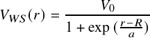
The modeling methodology [16] has been described in great detail in our previous paper on Shell model simulation [10]. So, only a brief description of the potentials rephrased in MeV and fm units are given here. In shell model, a nucleus of mass number A, consisting of N neutrons and Z protons has been modeled by the assumption that each nucleon experiences a mean field of central potential type due to rest of the nucleons. Woods-Saxon (WS) potential, which has typically a rounded square well shape, is one of the successful mathematical formulations graphically represented in Figure 2 and is given by

(1)

where 𝑉₀ is the depth of the well, given by [18]

𝑉0 =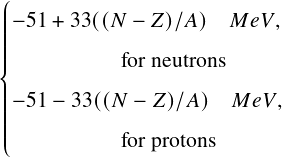

(2)

Here, r is the distance between two interacting nucleons, R is the radius of the nucleus, empirically obtained as N₀𝐴^1/3, with value of N₀ being 1.28, a is surface diffuseness parameter and is found to be 0.66 [10].]
Next, interaction of spin of nucleon with orbital angular momentum of nucleon, as confirmed in experiments [17], has been modeled by spin-orbit potential, as

(3)

Here, L.S =[𝑗(𝑗 +1)-ℓ(ℓ+1)-3/4]ℏ², where ℓ is orbital angular momentum quantum number, 𝑗 =ℓ+𝑠 is total angular momentum quantum number and 𝑠 is spin angular momentum quantum number given by 1/2 for nucleons. The model parameters are 𝑉₁ =-0.44𝑉₀ [18] and 𝑟₀ = 0.90, a proportionality constant optimised previously by our group [10] to obtain the right energy level sequence. In our earlier work [10], the parameters 𝑟₀ and 𝑎 were adjusted for a fixed value of N₀ during simulation to better match the experimental energy levels. It was found that for 𝑟₀ within range 0.86 - 0.95 and 𝑎 within range 0.66 - 0.67, the χ² value comes out to be minimum.
In case of protons, Coulomb potential also needs to be considered and is given by

(4)

Here N_𝑐 is the charge radius of the nucleus which in this case is considered to be equal to radius of nucleus R. The potential 𝑉_𝑐(𝑟) is to be rephrased in MeV units. So, it is multiplied and divided by electron rest mass energy, [19] 𝑚_𝑒𝑐² =0.511 MeV to obtain

(5)

The radial TISE for central potentials is given by

(6)

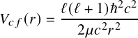
where V(r) is net interaction potential experienced by a neutron or a proton and second term inside bracket, resulting from solution of θ-equation, is called as centrifugal potential 𝑉_𝑐𝑓(𝑟) and μ is the reduced mass given by:

μ =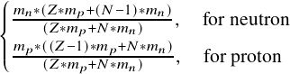

(7)

Here, 𝑚_𝑝 =938.272 and 𝑚_𝑛 = 939.565 are masses of proton and neutron respectively, in units of MeV/c². The centrifugal potential 𝑉_𝑐𝑓(𝑟) is rephrased in MeV units, by multiplying and dividing it by 𝑐², so that

(8)

The value of ℏ𝑐=197.329 MeV-fm.

3.   Numerical Solution

3.1.   Numerov technique in matrix form:

Consider TISE for a general potential V(r), given by

(9)

where

(10)

The advantage of this Eq. (9) is that it is linear in ’u’ having no first order derivative involved and is hence ideally suited for solving using Numerov method. The wave-function u(r) is expanded in Taylor series by explicitly retaining terms up-to 𝑂(ℎ⁴) and is obtained to an accuracy of 𝑂(ℎ⁶), [14]

𝑢(𝑟+ℎ)=𝑢(𝑟)+ℎ𝑢′(𝑟)+𝑢′′ (𝑟)+
𝑢′′′ (𝑟)+𝑢′′′′ (𝑟)+…		(11)

Discretizing x in steps of h as:
𝑟₁,𝑟₂,…,𝑟_𝑛-1,𝑟_𝑛,𝑟_𝑛+1,…,𝑟_𝑁 .
Here, 𝑟_𝑛 =𝑟₁ +𝑛×ℎ
Now expressing 𝑢(𝑟_𝑛 +ℎ) as 𝑢_𝑛+1, so on and similarly, 𝑘(𝑟_𝑛) as 𝑘_𝑛, Eq. (11) can be written as

𝑢𝑛+1 =+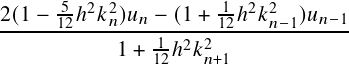
𝑂(ℎ6)		(12)

Substituting from Eq. (10), 𝑘_𝑛² =(𝐸-𝑉_𝑛) into the above, clubbing the terms containing 𝑉_𝑛 and 𝐸, it can be recast into the following form:

-+
		(13)
=𝐸		(14)

One has to keep in mind that whatever may be the potential, if wave-function were to be normalised, it should tend to 0 as x tends to ±∞. This implies, one has to choose the region of interest (RoI) large enough to ensure that the wave-function dies down to zero in either direction. That is, x values are limited to an interval such as [𝐿₁,𝐿₂], such that 𝑢 goes to 0 at both ends of the interval. More specifically,

(15)

and

(16)

Expanding the above equation for all intermediate points (𝑗 = 2,3,…,𝑁 -1), one will get a matrix equation as

(17)

where in, 𝑢 is a column vector (𝑢₂,…,𝑢_𝑛-1,𝑢_𝑛,𝑢_𝑛+1,…,𝑢_𝑁-1 ),
Similarly, V is a column vector (𝑉₂,…,𝑉_𝑛-1,𝑉_𝑛,𝑉_𝑛+1,…,𝑉_𝑁-1 ), but is converted into a diagonal matrix with these values along its central diagonal. Matrices A and B are given by

(18)

and

(19)

where 𝐼_𝑝 represents a matrix consisting of 1’s along 𝑝𝑡ℎ diagonal and zeros elsewhere, here 𝑝 can be positive (above the main diagonal, i.e 𝐼₁), zero (the main diagonal, i.e 𝐼₀) or negative (below the main diagonal, i.e 𝐼_-1).
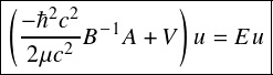
Multiplying Eq. (17) by B^-1 on both sides, gives TISE as a matrix equation, utilising Numerov method,

(20)

with an error of 𝑂(ℎ⁶).
Notice that a factor of 𝑐² is introduced in both numerator and denominator to ensure the units are in 𝑀𝑒𝑉 and 𝑓𝑚 as required in nuclear physics.
This is the final equation that needs to be solved numerically to get energy eigen-values and eigen-functions of a particle interacting with a given potential V(r). The imposition of boundary conditions as 𝑢₁ =𝑢_𝑁 =0 is equivalent to embedding the potential of interest, inside an infinite square well potential. Finally, (𝑁-2)×(𝑁 - 2) sub-matrices of A and B are utilised to solve for the energy eigen-values and their corresponding eigen-vectors.

4.   Algorithm for implementation in Gnumeric:

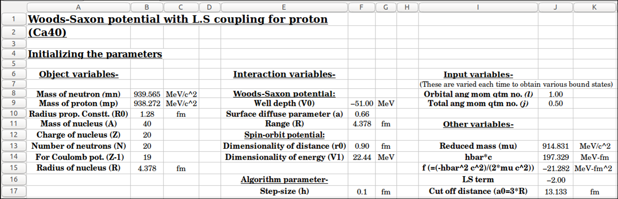
A step by step approach to determining the single particle energies for protons of ₂₀⁴⁰𝐶𝑎 is presented.

a)

Initialisation of parameters: There are two sets of parameters:

i.

Physical system parameters:
Object and interaction variables constituting as inputs and state variables which we wish to determine, are outputs. Figure (1) show object variables, interaction variables, Algorithm variables, input variables and other variables required for the calculations.

ii.

Algorithm parameters:
that arise from discretization of continuous variables and limiting the infinitely large quantities to finite values such as region of interest. The step size is chosen as ℎ=0.1 and is given in cell F17.

---

Figure 1: Initializing the parameters for the system

---

b)

Potential Definition:
First the values of ’r’ are generated from 0.1 to (3 ×N) with step-size ℎ=0.1 from A22 to A153, and to get the expected results, corresponding matrix size is 131 ×131. Then, four potentials are determined using the following formula for a particular ℓ and j values:

i.

Centrifugal potential 𝑉_𝐶𝐹 , in cell B22 type the formula:

                      =($J$8*($J$8+1)*$J$14^2*
           ($A22^(-2)))/(2*$J$13) 

ii.

Woods-Saxon potential 𝑉_𝑊𝑆 , in cell D22 by typing the formula:

          =$F$9*(1+$C22)^(-1)

iii.

L.S potential 𝑉_𝐿𝑆, in cell F22 by typing formula:

                      =-$F$14*$F$13^2*$J$16*$C22*
           $E22*($F$10*$A22)^(-1) 

where, the L.S term in cell J16 is calculated by formula:

          =$J$9*($J$9+1)-$J$8*
           ($J$8+1)-3/4

iv.

Coulomb potential, for proton, is given by typing formula:

                      =$B$14*0.511*2.839*
           (3*$B$15^2-$A22^2)/(2*$B$15^3) 

in cell G22 up-to radius ’R’ of the nucleus. After that in cell G65, type the formula:

          =0.511*2.839*$A65^(-1)*$B$14

---

Figure 2: (a) Total Interaction potential 𝑉(𝑟)= 𝑉_𝑐𝑓(𝑟)+𝑉_𝑊𝑆(𝑟)+𝑉_𝑙𝑠(𝑟)+𝑉_𝑐(𝑟) for proton (b) Plots of 1𝑠_1/2, 1𝑝_1/2 and 1𝑝_3/2 states for proton, showing the effect of Spin-orbit interaction in Woods-Saxon potential.

---

which gives the Coulomb potential outside the range of nuclear radius.

v.

In cell H22, the net potential is determined by typing the formula as:

                      =$B22+$D22+$F22+$G22 

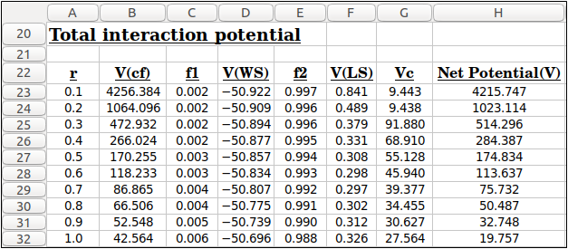
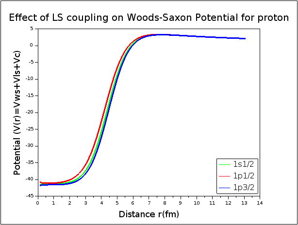
Figure (2a) consists of the potential values for the few r values and Figure (2b) shows the plot of Woods-Saxon potential of 1𝑠_1/2,1𝑝_1/2 and 1𝑝_3/2 states for proton, showing that inclusion of angular momentum on L.S coupling affects the Woods-Saxon potential.

c)

Determination of single particle energies:
This step consists of generating the following matrices and the same steps can be easily applied to matrix of any size.

i.

In Sheet 2, B-matrix is obtained as follows. Remember, B-matrix is constant for all problems. First generate index values for rows and columns as 1 to 5 from A43: A8 and B33: F3. In cell B4, the formula is given as

          =if($A4=B$3,10/12,
           if($A4+1=B$3,1/12,
           if($A4-1=B$3,1/12,0)))

This is repeated by dragging across till EB4 and then downwards to EB134 to obtain the tridiagonal B-matrix as shown in Figure (3a).

---

Figure 3: (a) Generating matrix-B (b) Generating matrix-B^-1 (c) Generating matrix-A (d) Generating matrix-B^-1*A (e) Generating matrix-V (f) Generating Hamiltonian matrix

---

ii.

In Sheet 3, the inverse of B, is obtained by selecting cells B43: EB134 and giving the formula as

                      =minverse(’Sheet 2’!B4:EB134) 

press Ctrl+Shift+Enter keys together to obtain matrix-𝐵^-1 as in Figure (3b).

iii.

In Sheet 4, A-matrix is generated similar to B-matrix, except that we need step size ’h’ from Sheet 1 available in cell F17, say.
Then, In cell D4, type =′𝑆ℎ𝑒𝑒𝑡1′!𝐹17.
In cell D3, insert the value of function 𝑓 = from cell J15 of Sheet 1. Then, in cell B7, the formula is given as

          =if($A7=B$6,(-2*$D$3/$D$4^2),
           if($A7+1=B$6,($D$3/$D$4^2),
           if($A7-1=B$6,($D$3/$D$4^2),0)))

and dragged appropriately to generate the required values as shown in Figure (3c).

iv.

To obtain matrix-𝐵^-1 *𝐴, in Sheet 5, select cells B4 : F8 and give formula:

                      =mmult(Sheet3!B4:EB134,’Sheet 4’!
          B7:EB137) 

The obtained matrix is shown in Figure (3d).

v.

Generate-V-matrix in Sheet 6, by giving the formula in cell B4 as

          =if($A4=B$3,’Sheet 1’!$H22,0)

so that only diagonal elements get populated as those of net potential values from Sheet 1 and seen in Figure (3e).

vi.

In Sheet 7, finally we generate the Hamiltonian matrix (i.e. matrix-𝐵^-1 *𝐴+𝑉) by simply giving the formula in B4 as

                      =(Sheet5!B4:EB134+’Sheet 6’
            !B4:EB134) 

and dragging the formula to fill values from B4: EB134 as seen in Figure (3f).

vii.

The main feature of Gnumeric which makes it different from other worksheet environments such as MS-Excel or open Office Calc. is that, it has an eigen-value solver.
Now, the eigen-values and corresponding eigen-vectors are obtained in Sheet 8 by selecting cells B4: EB135, a matrix of size 132 × 131, with an extra row to incorporate the eigen values. Each eigen vector of size 131 × 1 will be available below each of the eigen values in the first row. The formula is typed as

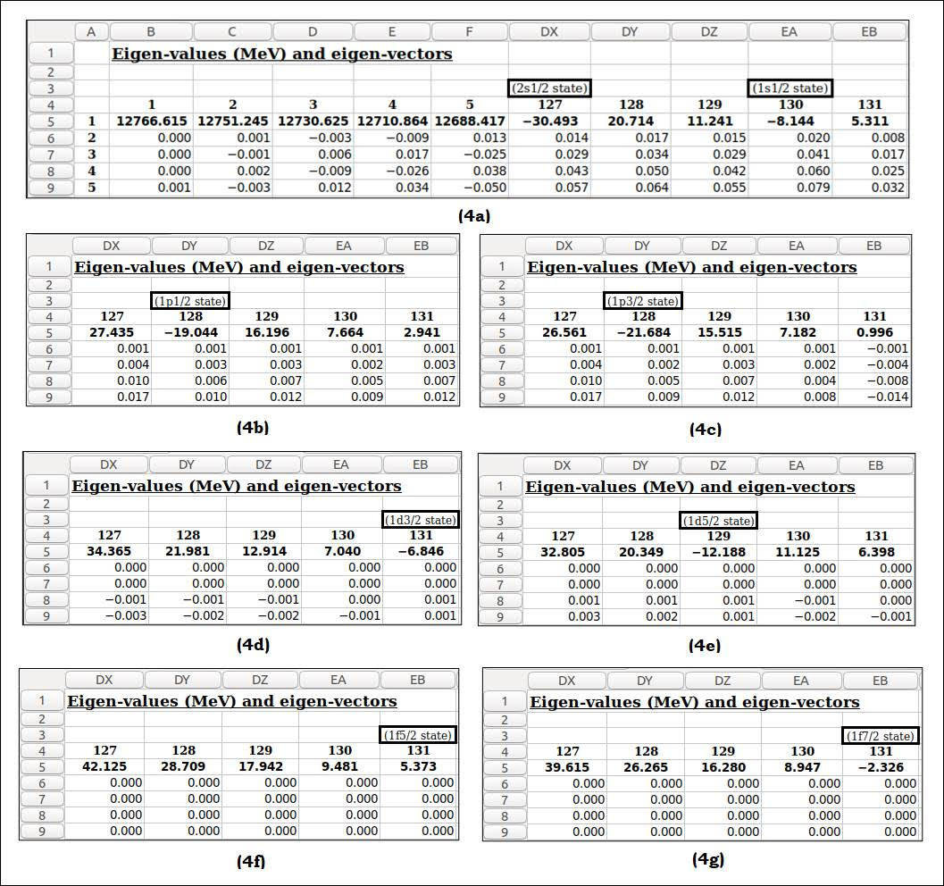
          =eigen(Sheet7!B4:EB134)

and all the three keys Ctrl+Shift+Enter pressed together. The resultant values are shown in Figure (4a) and (4b).

---

Figure 4: Calculation of eigen-values and eigen-functions

---

d)

Generating the energies for different ℓ and 𝑗 values: Now, the bound state energies, those for which eigen values are negative, are tabulated for different values of ℓ and 𝑗.

• Starting from ℓ =0, s-states, in which case 𝑗 =0.5 alone exists

• for ℓ = 1, p-states, we have two values of j: 𝑗 =0.5 and 𝑗 =1.5.

• Similarly for ℓ =2, d-states, 𝑗 takes values 1.5 and 2.5 , and so on.

This is continued till no bound states are obtained for particular ℓ and 𝑗 values.

5.   Results and Discussions:

In this section, we will first validate our approach to obtain energy eigen-values and eigen-functions using Woods-Saxon potential with 𝐿.𝑆 coupling for both neutron and proton for doubly magic nucleus ₂₀⁴⁰𝐶𝑎. This is done by comparing our results with available experimental results and those obtained numerically by using matrix method with Fourier basis [10] for different angular momentum values ℓ and j. The results are tabulated in Table 1.

The obtained energy eigen values are in good agreement with experimental energy values of different neutron and proton single particle states for step size of h=0.1 thus validating our approach. One can observe from the Table 1, that while the numerical or simulated values are below than those of experimental ones for lower proton and neutron states, the trend is opposite for higher states. This discrepancy arises because the optimization algorithm, in its attempt to minimize χ², tends to find values close to the expected ones.
The distance parameter ’r’ is discretized as per step size ’h’ and its values are varied from 𝑟 =0.1 to 𝑟 =3N, where N =N₀𝐴^(1/3). Therefore, it is necessary to vary the size of matrix ‘N’ for different A values for a chosen step size ‘h’. This simulation activity can be utilised as a tool to apply GIS[20] of constructivist approach to learning and has been done as follows:

5.1.   GIS Implementation:

The students have been taken through following six step process of GIS. All steps were implemented on online Moodle platform [21] during COVID-19 lockdown of university.

• Initiation: The matrix Numerov technique was already introduced before, for solving the harmonic oscillator potential. Next, it has been applied to solve for single particle energies of both neutrons and protons, as dealt with in this paper, for Woods-Saxon potential with spin-orbit potential. This has been explained and also demonstrated in two successive lab sessions.

• Selection: The students were made to explore the binding energy and separation energies curves that they have plotted in previous sessions, to identify various double magic nuclei suitable for study. The doubly magic nuclei from ₈¹⁶𝑂 to ₈₂²⁰⁸𝑃𝑏 were selected. The determination of single particle proton and neutron energy level sequences for six double magic nuclei, are assigned to students by dividing them into 12 groups. Each group is expected to obtain the energy level sequence of either neutrons or protons for the assigned nuclei by carefully following the simulation procedure.

• Presentation: The students in each group could be asked to present their findings to the rest of the class so that everyone gets to know each other’s experience. Even though all the groups could get to expected level sequence by following the steps correctly, some of the students have not ensured reduction of step-size systematically. Hence, they have come up with lower accuracy for energies even though they obtained correct level sequence. They have been guided accordingly.

• Exploration: The collective findings were shared with entire class and they were asked to explore nuclei adjacent to the magic numbers with one neutron or proton more and find out ground state 𝐽^π configuration for each of them.

• Formulation: They were expected to formulate their findings based on right choice of level sequence and also figure out what they would get if they followed the level sequence given in their prescribed textbook [4].

• Collection: To understand variation of energy level structure with mass number, students were asked to plot the compiled energy data for protons and neutrons as a function of mass number A. They were able to obtain plots similar to what have been presented in [10].

• Assessment: They have assessed their formulated ground state angular momentum and spin configurations based on the experimental findings and thus validated their outcomes. They could be further asked to obtain the ground state configurations of nuclei slightly away from magic nuclei till the results obtained are in variance with those from experiments as an excercise.

5.2.   Outcomes from GIS:

The results matching with experimentally available values [15] were obtained for step-size ’ℎ =0.1’ for doubly magic nuclei from ₈¹⁶𝑂 to ₈₂²⁰⁸𝑃𝑏. The value of N (to solve N × N matrix) for each of these nuclei are obtained as 96,131,138, 145, 177, 194 and 229 respectively. The obtained energy level sequences for neutrons and protons of these nuclei are given separately in tabular form in Tables 2 and 3. The first four levels, 1𝑠_1/2,1𝑝_3/2,1𝑝_1/2 ad 1𝑑_5/2 are not shown, as there are no discrepancies found in the ordering of these levels across the periodic table due to our simulation. The numerically obtained energy values are found to match to two decimal places with those obtained using the matrix method approach [10]. The χ²-value defined as relative mean-squared error

(21)

These are determined w.r.t experimental [15] and are shown in Tables. In Tables 2 and 3, energy level sequence obtained for lighter nuclei ¹⁶𝑂 to ⁵⁶𝑁𝑖 are shown in first column and that for ¹⁰⁰𝑆𝑛 to ₈₂²⁰⁸𝑃𝑏 in last column. It can be observed that the energy level sequence for lighter nuclei is different than that for heavier ones. This might be because the effect of spin-orbit coupling is different for light nuclei and heavy nuclei which results into the change in internal structure. Also, the amount of splitting in the energy levels is different for different mass numbers. The observed discrepancies in energy sequence are highlighted in red colour.
The discrepancy in level sequence for lighter nuclei w.r.t heavy nuclei is highlighted in blue colour in both tables; i.e for neutron and proton states. Further, it is found that in most of the textbooks at UG and PG level [4, 5, 6, 18, 22, 23], energy level sequence given is different. Also, there is only single energy level sequence given for both neutrons and protons, and that too common for all mass ranges. But according to our calculations as well as Bohr and Mottelson book, there should be different energy level sequences for nuclei across the periodic table.

Next, 𝐽^π assignments for nuclei near to doubly magic nuclei in mass range equal to and less than ₈₂²⁰⁸𝑃𝑏 based on our simulation, which match with experimentally[15] available energy sequence, are tabulated. These assignments are compared with those calculated using energy level sequence given in usually referred textbook Introductory Nuclear Physics by Kenneth Krane[4] by considering only the energy level sequence of lighter nuclei, and are shown in Table 4. The discrepancies in spin assignments are highlighted in blue colour. These discrepancies are also observed in other textbooks [5, 6, 17, 22, 23] as well.

Hence, from our observations, the level sequence for lighter mass range and heavy mass range nuclei can be modified accordingly so as to provide students with data consistent with experiments.

6.   Conclusion:

The time-independent Schrödinger equation (TISE) for a nucleus modeled using Woods-Saxon potential along with spin-orbit coupling term has been solved numerically by choosing Matrix Numerov method. The main advantage of matrix Numerov method is that it can be easily extended to any arbitrary potential of interest. It is implemented in Gnumeric worksheet environment to obtain numerical solutions of single-particle neutron and proton states for doubly magic nuclei ₂₀⁴⁰𝐶𝑎. Then, using guided enquiry strategy, a Constructivist approach, students were grouped and encouraged to obtain energy level sequences for other doubly magic nuclei up-to 𝑍 =82, i.e ₈¹⁶𝑂, ₂₀⁴⁸𝐶𝑎, ₂₈⁵⁶𝑁𝑖, ₅₀¹⁰⁰𝑆𝑛, ₅₀¹³²𝑆𝑛 and ₈₂²⁰⁸𝑃𝑏. Based on these obtained level structures, students obtained ground state total angular momentum and spin assignment for various nuclei close to doubly magic nuclei successfully and it could easily be extended to test the limits of validity.

References

Copyright

[© 2024 Shikha Awasthi, et al.] This is an Open Access article published in "Graduate Journal of Interdisciplinary Research, Reports & Reviews" (Grad.J.InteR³) by Vyom Hans Publications. It is published with a Creative Commons Attribution - CC-BY4.0 International License. This license permits unrestricted use, distribution, and reproduction in any medium, provided the original author and source are credited.

____________________________________________________________________________________________